During the last 10 years there has been a big and prolonged recession in the US. From the experience of previous business cycles, we would expect a rather quick recovery of actual output to its potential level – but not this time. Figure 1 shows that after a big contraction in 2008-2009 there is no fast recovery in the US. Instead, the growth rate seems to be permanently lower than before the contraction.
Hence, the questions we often hear today are: why do we have secular stagnation, where does it come from and what should we do about it?
Figure 1. US GDP normalized to equal zero in the first quarter of 2007
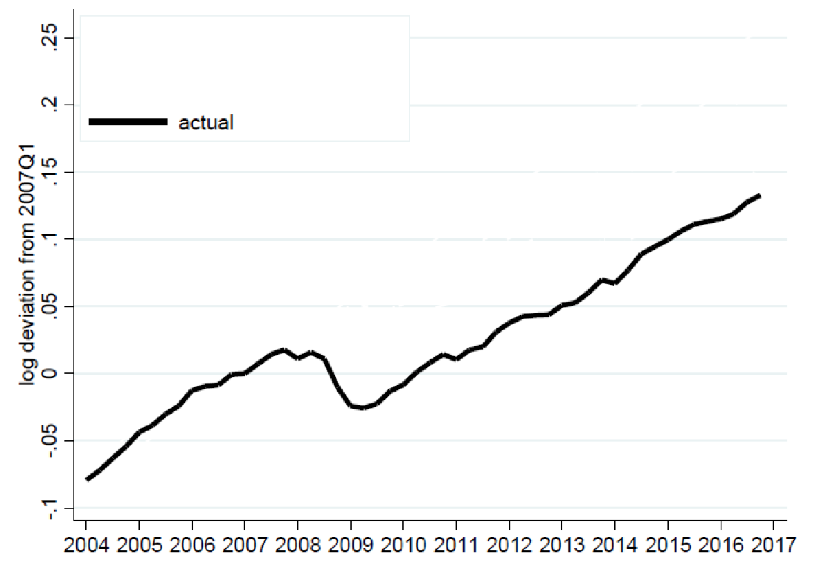
Figure 2 shows actual GDP (black line) contrasted to the dynamics of potential output calculated by the Congress Budget Office in 2007. This potential output line was produced just before the recession and was intended to show what was going to happen within the next 10-15 years. In a typical recession we would see convergence of the black line to the red line – but currently we don’t see it in the data. Instead, we see the conversion of potential output estimates to the actual output as the time passes (Figure 3).
Figure 2. Actual output dynamics vs potential output estimate produced by the Congress Budget Office (CBO) in 2007
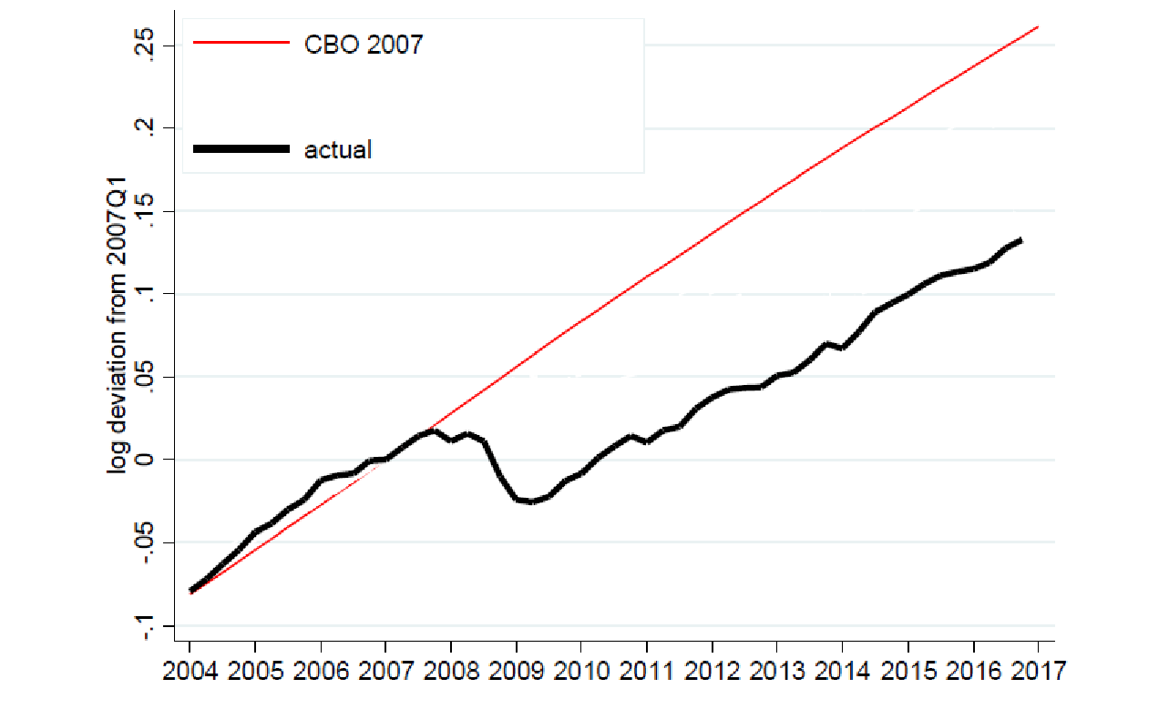
Figure 3. Actual output dynamics and revision of CBO estimates of potential output over time
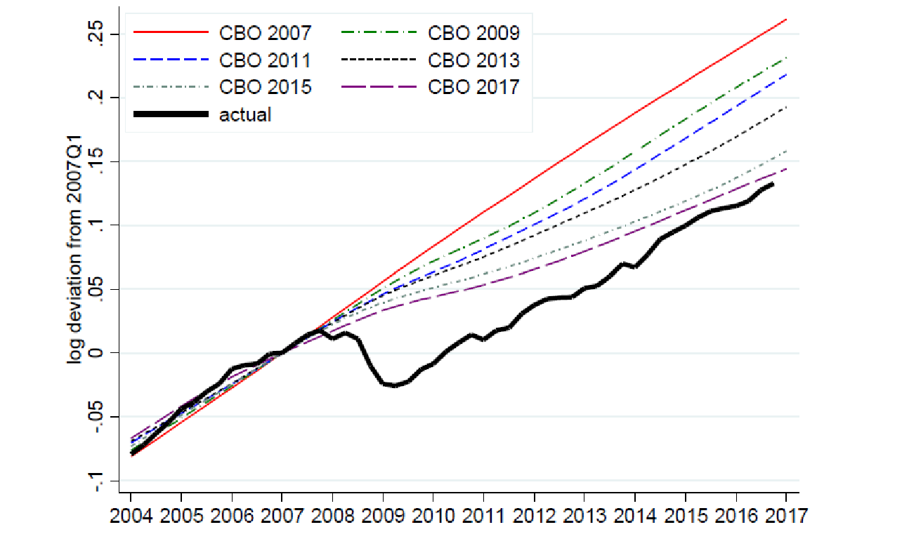
Today, as you see from the Figure 3, potential output is very close to actual output but it is closer not because the actual output caught up but because potential output estimate was revised downward.
It seems that now more and more people believe that we are in a state of very low output growth for a very long period of time.
What does this mean for central banks?
Many central banks are now using Taylor rule (1) or its modification to set policy rates.
it = i* + ϕπ(πt – π*) + ϕx(yt – yt*) (1)
where it is the central bank policy rate, i* is a natural (full employment) interest rate, πt and π* are current and expected inflation, yt are yt* are current and potential GDP growth, and ϕπ and ϕx are policy parameters.
The output gap (the distance between actual and potential output) is one of the key inputs into this policy rule (with the second key input being inflationary expectations). Therefore, for central banks potential output estimation is very important: if actual GDP is far below potential, a central bank will lower its policy rate or keep it low, if output is close to potential or above it, a central bank can raise its policy rate.
Therefore, the key questions for policy-makers are:
How much “slack” do we have in the economy? and
How permanent are the deviations from pre-crisis trends?
To answer these questions, we need to find out what we know about potential output estimates. And in particular, we need to answer the question of why we have revisions of potential output estimates.
Unfortunately, we know very little about how people come up with estimates of potential output and why they revise their estimates. Therefore the purpose of this paper is to come up with some very simple statistical framework to understand basic properties of potential output. This can be very helpful for understanding the implications for monetary policy: how does the distance between yt and yt* in the Taylor rule is moving in response to shocks?
To do that, we first collected measures of potential output for the US and other countries and then studied how identified shocks influence actual output and real-time estimates of potential output.
Our main results are that:
- Estimates of potential output respond to demand and supply shocks (while in theory potential output should respond only to supply-side shocks but not to transitory demand-side shocks)
- Potential output eventually catches up with actual output
- Properties of estimates of potential output can be well-approximated with one-sided univariate Hodrick-Prescott filter. This is the most striking result of our paper – that all these fancy models that provide potential output estimates can be very well approximated by a very simple statistical framework.
Hence, the decline in potential output is not necessarily as permanent as many academics and policy-makers think. It may be that we are just observing a bad shock that lasts for a long period, and nothing more.
Estimates of potential output
There are three main approaches to estimation of potential output:
- Production function.
Y* = f(K*, L*, productivity).
- Statistical approach.
Under this approach, one uses different methods to “clean” the data from transitory shocks and fluctuations, and then says that remaining long-term trend is the potential GDP.
- Structural approach (the most sophisticated one).
One estimates a structural model of the economy (e.g. a dynamic general equilibrium model), and in this model the potential output is the output when transitory shocks and frictions are “turned off”.
Data sources
There are several sources of potential output estimates:
- Congress Budget Office (CBO), which is the US “golden standard” for these estimates. It uses the production function approach, and its data extend back to 1991
- Estimates of Federal Reserve Board (Greenbook) used for setting monetary policy. They use a variety of methods including judgmental method when some experts look at the data and try to use information which is not necessarily in the models to make sure that they have the best possible estimate. This sample ranges from 1987 to 2011 (they release the information with a five-year delay)
- The IMF, which also uses a mix of methods including judgmental. The key advantage of this source is that it has the estimates for many countries so we can use not only time series variation but also cross-sectional variation of potential output estimates.
- OECD also uses a production function approach and provides the data for a large number of countries for a long period of time.
- Private sector estimates (since private forecasters do not produce potential GDP estimates, we use their long-term – up to 10 years – forecast of actual GDP)
Stylized facts
Before going into further analysis, let me provide you with a few stylized facts about the potential GDP estimates.
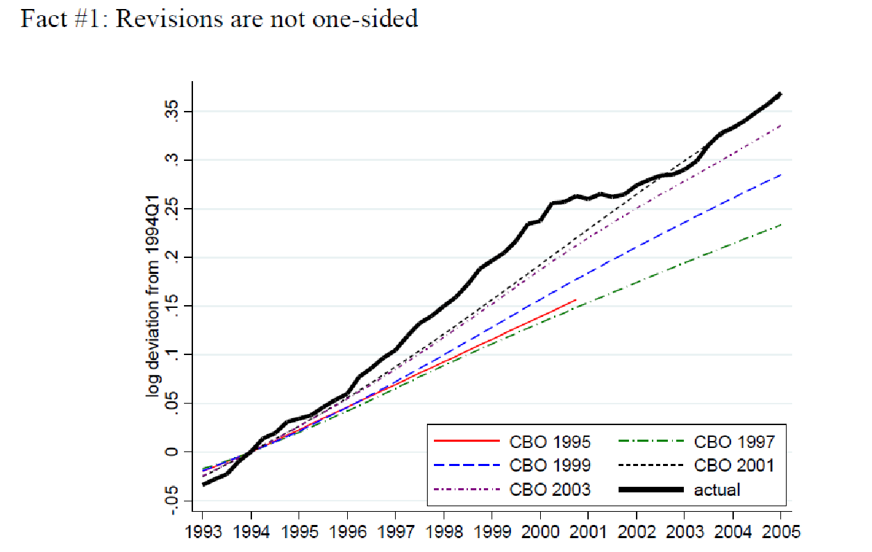
First, potential GDP revisions can be both negative and positive. An example of a positive revision is the second half of 1990s, when US economy was growing really fast (Figure 4).
Figure 4. revisions of potential GDP in 1993-2005
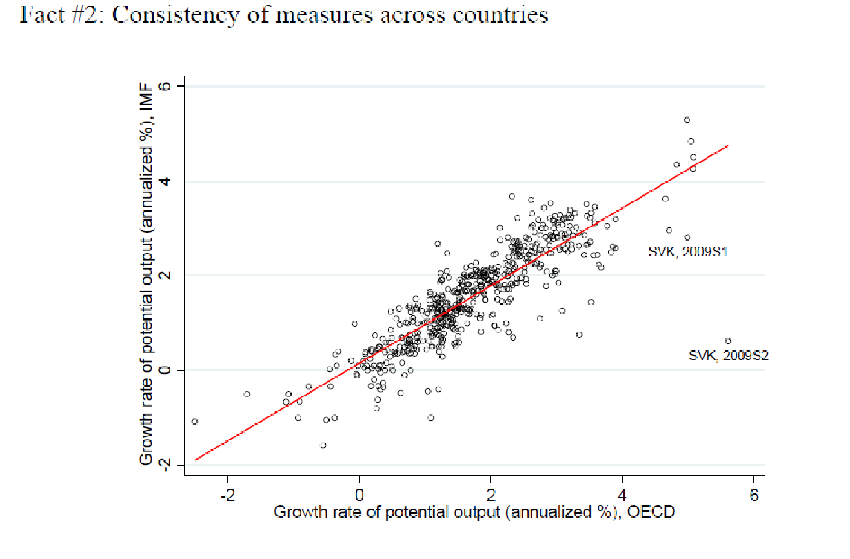
The second fact is that there is a lot of consistency in the estimates of potential output across sources. Figure 5 shows that the correlation between potential output measures calculated by OECD and the IMF is very tight – about 0.99. So it seems that there is a lot of agreement in how people calculate potential output across those different agencies.
Figure 5. Correlation between IMF and OECD estimates of potential output growth
There is consistency between estimates of different agencies not only across countries but also across time (figure 6). Figure 6 also suggests that measures of potential output considerably fluctuate over time.
Figure 6. Potential output measures from different agencies across time within countries
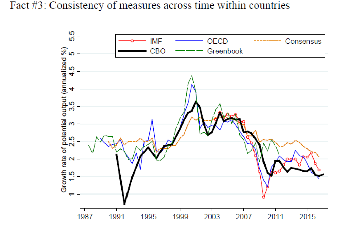
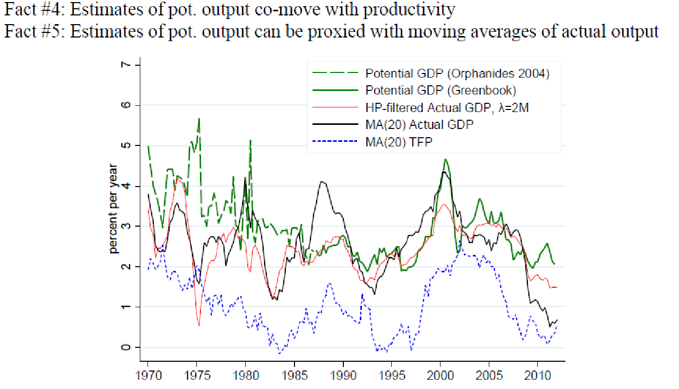
Figure 7 illustrates two final stylized facts: that estimates of potential output are highly correlated with changes in productivity (the green line and the blue line in Figure 7) and that estimates of potential output can be very well proxied by moving averages of actual output (red line and black line).
Figure 7. Comparison of estimates of potential output with productivity growth and smoothed actual output
Results
Now we test how estimates of potential output react to different types of shocks. To do that, we estimate OLS regressions with changes in potential output as a dependent variable and derive impulse response functions for them.
In theory, potential output should respond to permanent shocks, which are supply side shocks. The examples of such shock are (1) a rise in productivity – for example, an improvement in technology; (2) a permanent change in taxation regime – e.g. if there is an income tax cut, people will start to work more; (3) an oil price shock – since the elasticity of demand for energy is low, a change in oil price will impact productivity.
In contrast, demand-side shocks which are driving business cycles are transitory and thus should not impact the estimates of potential output. Examples of demand-side shocks are (1) monetary policy shocks – e.g. a change in central bank policy rate; (2) a change in government spending (e.g. a rise in military spending).
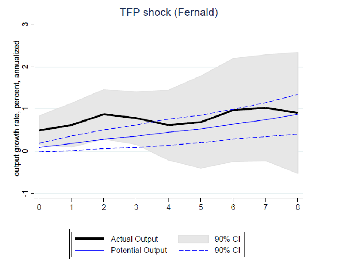
Figure 8 shows a reaction of actual (black line) and potential output (blue line) to the TFP shock. We see that actual GDP increases right after the shock and then stays at some permanently higher level. We would expect the same dynamics from potential output. Instead, we observe a gradual increase in potential output until the output gap is closed. You can do this exercise with other supply shocks as well.
Figure 8. Impulse response function to a permanent supply shock (a TFP increase)
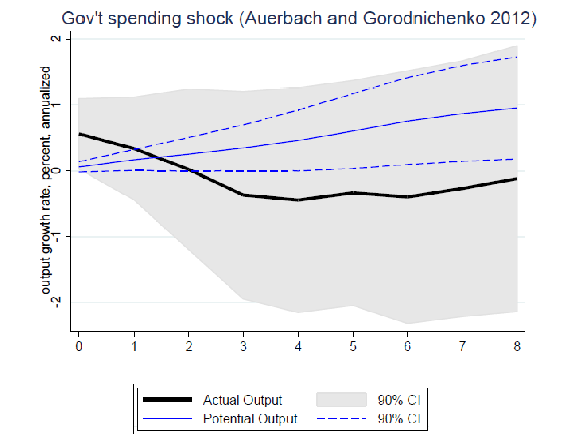
Here is an example of a demand-side shock (Figure 9) – an unanticipated decline in government spending. The actual output declines at first but quickly returns to the long-term trend. Potential output does not react to the shock at first, but then it starts to increase, which is really counterintuitive. Potential output should not react to transitory demand shocks.
Figure 9. An impulse response function to a government spending shock
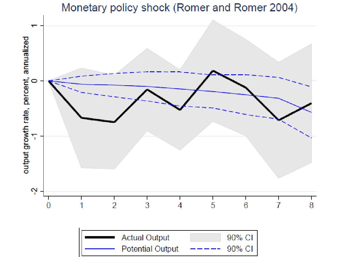
Another very good example is a monetary policy shock (Figure 10). If you have monetary tightening, at first the actual output does not react but then there is some contraction. The striking thing here is that potential output is also moving quite strongly in response to the shock while it shouldn’t be doing this because, as we know, monetary policy shocks are transitory and they do not influence productive capacity of the economy.
Figure 10. impulse response functions of actual and potential GDP to a monetary policy shock (e.g. an interest rate increase)
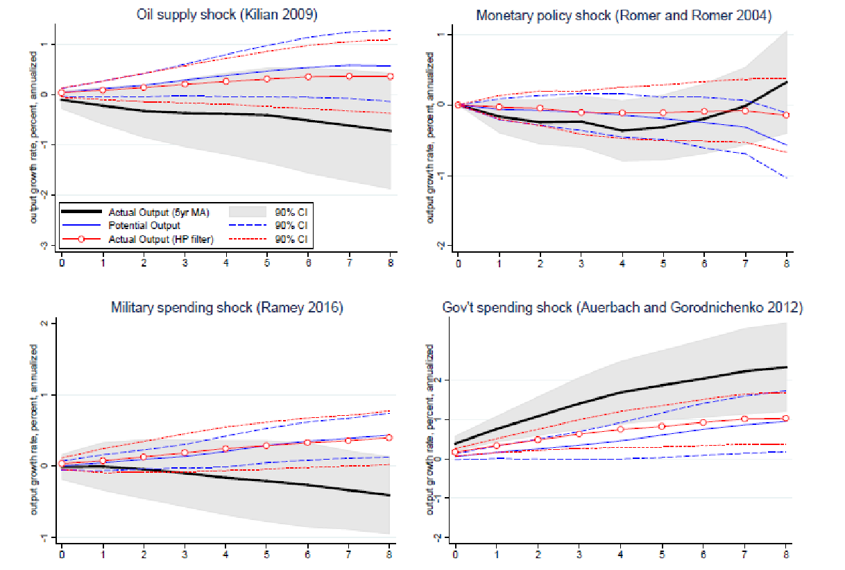
After getting these striking results, we decided to investigate, why potential output reacts albeit sluggishly but strongly to all the shocks. So we repeated the exercise for HP-filtered actual output series, and we observe that responses of these series to both supply and demand shocks are not statistically different from responses of our measures of potential output (in the Figure 11 red line is very close to the blue line).
Figure 11. Impulse response functions for actual output, potential output and HP-filtered actual output
We do a similar exercise for cross-country data and get very similar results.
Conclusions
Both private and public estimates of potential GDP respond gradually but systematically to all of the economic shocks that we consider and they deviate little from what one would expect from simple univariate time series estimates of potential GDP.
The fact that private and public forecasters now attribute much of the decline in output across countries since the Great Recession to changes in potential GDP tells us potentially little about whether these changes in output are in fact likely to persist or whether they can be reversed through monetary or fiscal policies.
Hence, there is a need to use additional macroeconomic variables to better identify supply and demand shocks rather than relying on univariate processes. It is also good to combine information from public estimates of potential GDP with private sector forecasts, as the latter appear to be somewhat more successful in isolating supply shocks from demand shocks. When estimating potential GDP, one needs to avoid excessive use of model-averaging since these mechanically induce movements in estimates of potential GDP after cyclical demand-driven fluctuations.
More generally, the absence of clear ways to successfully estimate potential GDP suggests that the practice of relying on “judgement” by professional economists should not be discontinued any time soon.
Question: I think that one implication of your results is that US government and other governments should continue expansionary monetary and fiscal policies since today actual output probably is not close to potential as the CBO estimates suggest. Reversal of expansionary policy today can prolong stagnation.
Answer: I agree that one interpretation of our results is that the notion of no slack in the economy now maybe a purely statistical result. And there are some signals consistent with the sense that we have a lot of slack in the US economy – for example, employment to population ratio has not recovered to the pre-recession level yet. However, there is a range of alternative interpretations consistent with our results. What we find very striking is that we often literally calculate the distance between actual and potential output and build policy around that. Our paper shows that the construct that we call potential output requires a very careful interpretation – it is not necessarily the true potential output.
Main photo: depositphotos.com / tycoon
Attention
The authors do not work for, consult to, own shares in or receive funding from any company or organization that would benefit from this article, and have no relevant affiliations