The theme of this paper is very close to the main issue central bankers are concerned with, which is keeping inflation low, predictable and stable. Central bankers are aware that stabilizing inflation often comes at the cost of destabilizing output and employment. These relationships are often referred to as the Philips curve.
If you look at actual macro data, you will see that inflation tends to be relatively stable when there are disturbances in the economy, so you would say that Philips curve is flat. This is surprising because when you look at micro data, you would see that not all prices adjust. Prices are sticky – i.e. they tend to stay fixed for a certain period of time (a few months). On average, about once a year a given price would change.
If you write a model that simulates the decision of adjusting price infrequently by retailers (a model that would match this microdata) – that model would actually fail to match the macro fact of the flat Philips curve. This puzzle – the disconnect between evidence from micro data and macroeconomic conclusions – generated a lot of literature that tries to solve it.
Theorists had to add new features to the models used by central bankers and macroeconomists:
- imperfections in goods markets or product markets;
- imperfect or incomplete information available to firms that adjust prices;
- price adjustment mechanism (price selection), which is the focus of our paper.
Retailers change not all but only some prices at any point in time – and we focus on how they make this decision, how they choose which prices to adjust.
Price selection exists when prices that are changed at any given point in time are not representative of the population of the prices in the economy. For example, think of a nominal unexpected expansion in the economy that pushes all prices upwards. If at that time prices that do adjust tend to be lower than the average representative price, then price changes tend to be larger than otherwise would be, and hence the inflation response is more sensitive to this underlying disturbance.
To explain it in more detail, I will provide examples of two very popular models of inflation fluctuations used in the literature. These two models provide two different extreme views on price selection mechanism.
The first model implies no price selection (time-dependent price adjustment; Calvo, 1983). This is a very popular model often used by central bankers in their inflation forecasts.
Think of a very simple world where there is one generic good, all retailers are the same and change prices not frequently but from time to time because they have to pay a cost every time they adjust the price.
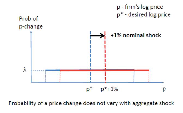
Figure 1. Time-dependent adjustment (Calvo model)
If they did not face any cost of adjusting prices, they would set prices to the desired price level p* immediately but since they have to pay the cost, sometimes they do not adjust the price – so with time their prices are further and further away from the desired level. In the Figure 1, the distance between the price of a given retailer and p* presents potential benefit for a retailer of adjusting that price to the desired level – so the further away the price on this domain (the bold black line in Figure 1) is from the p*, the bigger is the benefit of adjusting this price for a retailer.
The assumption made in the Calvo model is that the probability (λ) of adjusting any given price does not depend on how valuable it would be to adjust the price for this retailer (i.e. the probability is independent of current price). So if there is a nominal shock that pushes p* up by 1% (red lines in Figure 1), the probability of adjustment does not change. Any price in a store has the same probability of being adjusted, so it is representative of the population – and this illustrates zero price selection.
The second model implies a substantial amount of price selection (state-dependent price adjustment).
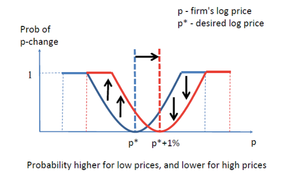
Figure 2. State-dependent adjustment (Golosov-Lucas, 2007)
In this model adjustment depends on a given price. The probability of adjustment is close to zero when current price p is close to the desired price p*, since for a retailer the cost of adjustment is bigger than the benefit. For prices that are further away from p*, the benefit of adjustment becomes higher than the cost, and so the probability of price change increases.
Let’s see what happens after the same shock which pushes prices up by 1%. In this model, when p* shifts to the right, the whole probability curve shifts as well (since it is centered on p*). Then for prices to the left of p* (i.e. for lower prices) the probability of adjustment goes up after the shock. And for prices that were high relative to p*, the probability of adjustment after the shock is going be lower because p* now becomes closer to the actual price.
On the aggregate level, lower prices mostly adjust to the shock while high prices do not – so aggregate price level tends to go up. This price selection mechanism makes the aggregate price level to adjust more sensitively to the original shock.
In this paper we propose a mechanism to identify price selection in the data and we see how important price selection is for inflation sensitivity.
We find that prices that adjust are more or less representative of the average price, potentially pointing us to the Calvo model.
We use microdata on prices on a number of goods in the UK. The dataset covers about 60% of consumption basket of British consumers. We have 13 months of time span and nearly 17 million observations.
Define pit the log price of a good i in a period t. Then inflation (πt) is just a weighted average of price changes between periods t-1 and t.
πt=iωit(pit-pit-1)iωit
Inflation can be split into two multiples – the fraction of prices that change (because not all prices change) – extensive margin, and the average size of change (intensive margin). When calculating the intensive price margin, we normalized the price change of each good by the average price of goods of this category.
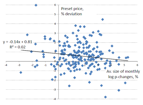
The main hypothesis that we are testing is how much the fluctuations in the preset price level (i.e. the price in the period t-1) contribute to fluctuations in the average size of price changes. In the Calvo model, the correlation between the two would be zero.
Other lectures at the NBU Conference
Taylor Rules versus Discretion in U.S. Monetary Policy. A Lesson for Ukraine, lecture by Alex Nikolsko-Rzhevskyy
Prudential Regulation: Are Government Bonds Safe, lecture by Igor Livshits
We exclude sales prices, control for seasonality, recession, tax changes etc. but our findings are robust to the “noise” in the data.
Main findings:
- inflation fluctuations are mostly explained by intensive margin (by average size of price changes);
- correlation between variations in average size of price changes and preset price level is very low (up to 0.16) – see Figure 3;
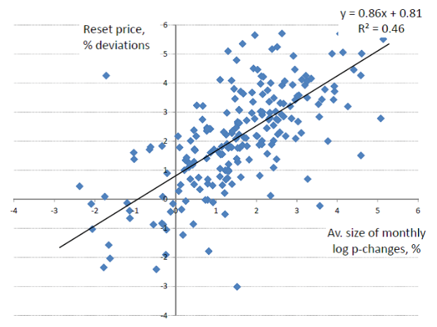
- correlation between variations in average size of price changes and reset price level (i.e. price level at time t) is quite high – Figure 4.
Figure 3. Correlation between variations in average size of price adjustment and preset price
Figure 4. Correlation between variations in average size of price adjustment and reset price
So, for now we find more support for Calvo model – we do not see much price selection in the data.
The bottom line of this paper is that the models with weak price selection that central banks are currently using are probably the right models to use to forecast inflation.
VoxUkraine is grateful to Yaroslav Kudlatskiy for writing down this lecture
Lecture by Oleksiy Kryvtsov at the NBU conference on May 19-20, 2016. Based on the forthcoming paper by Oleksiy Kryvtsov and Carlos Carvalho.
The views expressed here are my own and not of the Bank of Canada
Attention
The authors do not work for, consult to, own shares in or receive funding from any company or organization that would benefit from this article, and have no relevant affiliations
